Sentry Page Protection
Lesson 24: Differentiation Rules for Exponential Functions
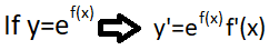
Exponentials and their derivatives have many applications in engineering, mathematics, science, and business studies. In this lesson, we will be dealing with derivatives of exponential functions that are more complex. All differentiation rules apply to exponential functions, including the chain rule. Remember, approach the problems from outside in, applying all relevant differentiation rules. Let us begin with a few problems:
Take the derivative of the following function.
Take the derivative of the following function.

First we will note that we are dealing with a product of functions. The first function we are dealing with is 3e^x and the second function we are dealing with is cos x. As a result, we will have totroy boy utilize the product rule, moving from outside in and applying all other relevant differentiation rules:
f(t)=(3e^x)(cos x)
f'(t)=d/dt(3e^x)(cos x) + (3e^x) d/dt(cos x) Apply the product rule.
f'(t)=(3e^x)(cos x) + (3e^x)(- sin x) Note that the derivative of 3e^x is 3e^x.
f'(t)=(3e^x)(cos x) - (3e^x)(sin x)
f'(t)=(3e^x)(cos x - sin x)
Let us run through another similar problem.
Take the derivative of the following function:

We notice that the above is a difference of functions, so we do not have to apply the difference rule. Before we differentiate it is important to note that differentiation of e^x gives e^x, the exact same function. Note that we can replace the variable x with anything and the derivative would still be exactly the same. Therefore we can summarize:
So in the function above the derivative of e^-x would still give us e^-x. However, we note that -x is a function, so we will have to utilize chain rule because the exponent is not simply x, but a distinct function, -x.
f(t)=e^(x)-e^(-x)
f'(t)=e^(x)-e^(-x)(-1) We use the difference rule as well as the chain rule.
f'(t)=e^(x)+e^(-x)
f(t)=e^(x)-e^(-x)
f'(t)=e^(x)-e^(-x)(-1) We use the difference rule as well as the chain rule.
f'(t)=e^(x)+e^(-x)
We already know that local maxima and minima are local extrema and that they can be found using the first derivative because a local extrema separates alternate sections of increase and decrease. Let's run through a problem where we are asked to determine the local extrema.
Given the following function, determine all local extrema.
Given the following function, determine all local extrema.

We know that the slope is zero at local extrema. Let us take the first derivative of the function, equate it with zero and solve.
f(x)=x³(e^x)
f'(x)=d/dx(x³)(e^x)+x³d/dx(e^x)
f'(x)=(3x²)(e^x)+x³(e^x)
f'(x)=(3x²)(e^x)+x³(e^x)
f'(x)=(x²)(e^x)[3+x]
0=(x²)(e^x)[3+x]
There are 3 cases because the equation above has 3 factors. Solve for x in each case, if possible:
Case 1:
x²=0 Take the square root of both sides.
x=0
Case 2:
(e^x)=0
We already know that the graph of y=e^x never touches the x-axis because it has an asymptote at the x-axis. Therefore this case has no solution.
Case 3:
3+x=0
x=-3
The two solutions occur at x=0 and at x=-3. To verify that they are local maxima and minima verify test points over all intervals created. Three intervals have been created:
Interval 1 (for x<-3)
Interval 2 (for -3<x<0)
Interval 3 (for x>0)
Verify the value of each interval to see if it is an interval of increase or decrease:
For Interval 1 (test x=-4):
f'(x)=(x²)(e^x)[3+x]
f'(-4)=((-4)²)(e^(-4))[3+(-4)]
f'(-4)=-0.29
For Interval 2 (test x=-1):
f'(x)=(x²)(e^x)[3+x]
f'(-1)=((-1)²)(e^(-1))[3+(-1)]
f'(-1)=0.74
For Interval 3 (test x=1):
f'(x)=(x²)(e^x)[3+x]
f'(1)=((1)²)(e^(1))[3+(1)]
f'(1)=10.8731
Because Interval 1 is decreasing (the derivative is negative) and Interval 2 is increasing (the derivative is positive) we can summarize that there exists a local minimum at x=-3. Also, because Interval 2 and Interval 3 are both increasing, there exists no local extrema between them. To solve for the local minimum, plug in x=-3 into the original function.
f(x)=x³(e^x)
f(-3)=(-3)³(e^-3)
f(-3)=(-27)(e^-3)
f(-3)=(-27)/(e^3)
Therefore the only local extrema of the function f(x)=x³(e^x) is a local minimum at (-3, -27/(e^3)). Next we will look at a problem where depreciation is modelled. Exponential functions are useful for modelling depreciation.
Joe decides that he wants to purchase a new car for $20,000. The value of the depreciating car over time can be modelled by the function below, where V(t) represents the value of the car and t represents the time in years after the initial purchase. Determine the rate of depreciation of the car at the time that it is driven off the dealer lot. Suppose that Joe will stop collision coverage on the car's insurance as soon as the value hits one-fifth of the original value. When will Joe stop collision coverage? Also, at what rate is the car depreciating when Joe stops collision coverage?
f(x)=x³(e^x)
f'(x)=d/dx(x³)(e^x)+x³d/dx(e^x)
f'(x)=(3x²)(e^x)+x³(e^x)
f'(x)=(3x²)(e^x)+x³(e^x)
f'(x)=(x²)(e^x)[3+x]
0=(x²)(e^x)[3+x]
There are 3 cases because the equation above has 3 factors. Solve for x in each case, if possible:
Case 1:
x²=0 Take the square root of both sides.
x=0
Case 2:
(e^x)=0
We already know that the graph of y=e^x never touches the x-axis because it has an asymptote at the x-axis. Therefore this case has no solution.
Case 3:
3+x=0
x=-3
The two solutions occur at x=0 and at x=-3. To verify that they are local maxima and minima verify test points over all intervals created. Three intervals have been created:
Interval 1 (for x<-3)
Interval 2 (for -3<x<0)
Interval 3 (for x>0)
Verify the value of each interval to see if it is an interval of increase or decrease:
For Interval 1 (test x=-4):
f'(x)=(x²)(e^x)[3+x]
f'(-4)=((-4)²)(e^(-4))[3+(-4)]
f'(-4)=-0.29
For Interval 2 (test x=-1):
f'(x)=(x²)(e^x)[3+x]
f'(-1)=((-1)²)(e^(-1))[3+(-1)]
f'(-1)=0.74
For Interval 3 (test x=1):
f'(x)=(x²)(e^x)[3+x]
f'(1)=((1)²)(e^(1))[3+(1)]
f'(1)=10.8731
Because Interval 1 is decreasing (the derivative is negative) and Interval 2 is increasing (the derivative is positive) we can summarize that there exists a local minimum at x=-3. Also, because Interval 2 and Interval 3 are both increasing, there exists no local extrema between them. To solve for the local minimum, plug in x=-3 into the original function.
f(x)=x³(e^x)
f(-3)=(-3)³(e^-3)
f(-3)=(-27)(e^-3)
f(-3)=(-27)/(e^3)
Therefore the only local extrema of the function f(x)=x³(e^x) is a local minimum at (-3, -27/(e^3)). Next we will look at a problem where depreciation is modelled. Exponential functions are useful for modelling depreciation.
Joe decides that he wants to purchase a new car for $20,000. The value of the depreciating car over time can be modelled by the function below, where V(t) represents the value of the car and t represents the time in years after the initial purchase. Determine the rate of depreciation of the car at the time that it is driven off the dealer lot. Suppose that Joe will stop collision coverage on the car's insurance as soon as the value hits one-fifth of the original value. When will Joe stop collision coverage? Also, at what rate is the car depreciating when Joe stops collision coverage?
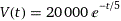
To find the rate of change when the car is driven off the dealer lot, take the value function and differentiate it. Then solve for t=0:
V(t)=20000(e^(-t/5)) Utilize the chain rule and the constant multiple rule.
V'(t)=20000(-1/5)(e^(-t/5))
V'(t)=(-20000/5)(e^(-t/5))
V'(t)=(-4000)(e^(-t/5))
Now solve for t=0:
V'(0)=(-4000)(e^(-(0)/5))
V'(0)=-4000(1)
V'(0)=-4000
When Joe drives the car off the car was depreciating at a rate of $4000 per year. To determine when Joe will stop collision coverage we must determine when the value of the car hits one fifth of its original value. This means we need to figure out when the value of the car hits $4000 because this represents one fifth of the original purchase price of $20,000. Let V(t) equal 4000 and solve for t:
V(t)=20000(e^(-t/5))
4000=20000(e^(-t/5))
4000/20000=(e^(-t/5))
0.2=(e^(-t/5))
ln 0.2=ln (e^(-t/5)) At this point take the natural logarithm of both sides. Remember ln (e^x)=x.
ln 0.2=-t/5 Because ln (e^x)=x, ln (e^(-t/5))=-t/5.
t=-5 (ln 0.2)
t≃8.0
Therefore Joe will stop collision coverage after 8 years. Next, we must find the rate of depreciation when collision coverage is stopped,. To do this take the exact value for the time when Joe stops collision coverage, t=-5 (ln 0.2), and plug it into the derivative of the original function.
V'(t)=(-4000)(e^(-t/5))
V'(-5 ln 0.2)=(-4000)(e^(-(-5 ln 0.2)/5))
V'(-5 ln 0.2)=(-4000)(e^(ln 0.2)) Remember, e^ ln x = x. Therefore e^(ln 0.2) = 0.2.
V'(-5 ln 0.2)=(-4000)(0.2)
V'(-5 ln 0.2)=-800
Therefore when Joe stops coverage after eight years, the car is depreciating at a rate of $800 per year. That's all there is to this lesson. Next lesson we will look at applications of exponential models in the everyday world.
© 2020 MyMathEducator.com All Rights Reserved